
In this post, we will continue our journey into search with Splunk and add a few more commands to include in your arsenal of knowledge. Please revisit our previous posts to ensure you have a healthy environment upon which to run commands.
Prerequisite
How to Install Splunk on Linux
Upload data required for the examples in this post.
- Download Tutorials.zip and Prices.csv.zip to your machine.
- Log in to Splunk Web. Go to Settings. On the settings page click on Add Data in the left pane.
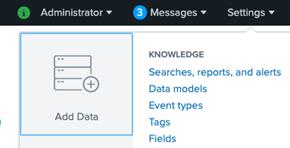
- On the Add Data page click on the Upload
- On the file upload page select or drag and drop files/archives that you have downloaded (one-by-one). You do not have to extract the archive.
- After the upload is finished click on Next.
- Select the source type as “Auto.”
- In the Host name extract field, use the Segment with value as 1 if you have Splunk running on Linux system. If you have Splunk running on Windows system use regular expression-based extract with regex value as \\(.*)\/.
- Create and select a new Index “test.”
- Complete the upload for both the files.
Searching and filtering
Commands in this category are used to search for various events and apply filters on them by using some pre-defined criteria.
Searching and filtering commands:
- Search
- Dedup
- Where
- Eval
Search
The search command is used to retrieve events from indexes or to filter the results of a previous search command in the pipeline.
You can retrieve events from your indexes by using keywords, quoted phrases, wildcards and key/value expressions.
The search command is implied at the beginning of any search. You do not need to specify the search command at the beginning of your search criteria.
Order does not matter for criteria.
index=test host=www* |
Is the same as
host=www* index=test |
Quotes are optional for search command, but you must put quotes when the values contain spaces.
index=test host=”Windows Server” |
Dedup
The dedup command removes the events that contain an identical combination of values for the fields that you specify.
With dedup, you can specify the number of duplicate events to keep for each value of a single field or for each combination of values among several fields. Events returned by dedup are based on search order.
Remove duplicate search results with the same host value.
index=test | dedup host |
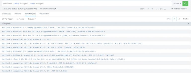
Get all user agents under index test.
index=test | dedup useragent | table useragent |
Where
The where command performs arbitrary filtering on the data and uses eval expressions to filter search results. The search keeps only the results for which the evaluation was successful (that is, the Boolean result = true).
The where command uses the same expression syntax as the eval command. Also, both commands interpret quoted strings as literals. If the string is not quoted it is treated as a field name. Use the where command when comparing two different fields, as this cannot be done by using the search command.
Command | Example | Description |
Where | … | where foo=bar | This search looks for events where the field foo is equal to the field bar. |
Search | | search foo=bar | This search looks for events where the field foo contains the string value bar. |
Where | … | where foo=”bar” | This search looks for events where the field foo contains the string value bar. |
Example-1:
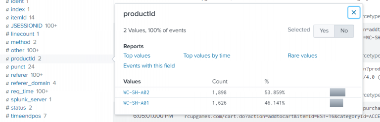
Find the events with ProductID starts with the value WC-SH-A.
index=test | where like(productId, “WC-SH-A%”) |
You can only specify a wildcard (% sign) with the where command by using the “like” function.
Example-2:
Search the events with failed HTTP response (HTTP response status can be found with field name status).
index=test | where status!=200 |
Eval
The eval command is used to add new fields in the event by using existing fields from the event and arbitrary expressions. The eval command calculates an expression and puts the resulting value into a search results field.
If the field name that you specify does not match a field in the output, then a new field is added to the search results.
If the field name you specify matches a field name that already exists in the search results, then the results of the eval expression overwrite the values for that field.
The eval command evaluates mathematical, string, and boolean expressions.
Example-1:
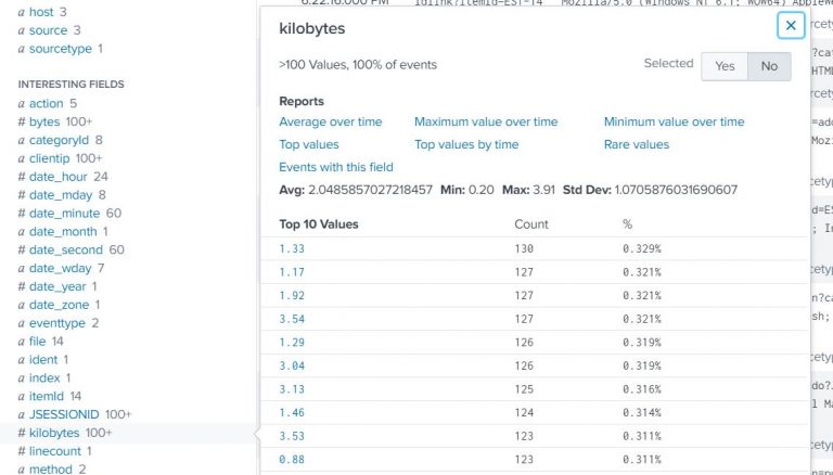
Convert the response size from bytes into kilobytes (tutorials data (sourcetype=access*) consisting of web server logs that contain a field named bytes, which represents the response size).
index=test sourcetype=access* | eval kilobytes=round(bytes/1024,2) |
Example-2:
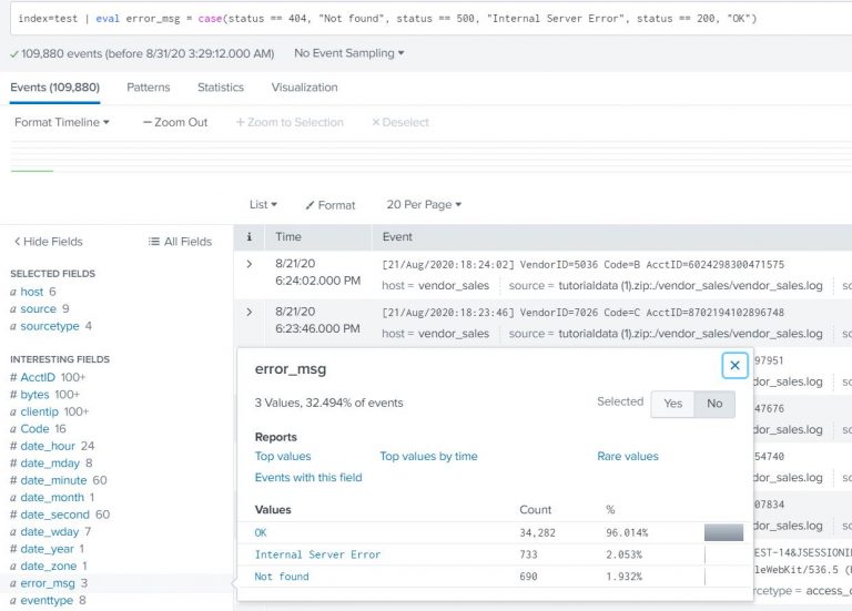
Create a field called error_msg in each event. Distinguish the requests based on the status code. Status 200 is okay, 404 is page not found, 500 is an internal server error (hint – use case statement with field status).
index=test | eval error_msg = case(status == 404, “Not found”, status == 500, “Internal Server Error”, status == 200, “OK”) |
Formatting and ordering
These commands are used to reformat the search results and order them based on the field values.
Formatting and ordering commands:
- Rename
- Table and Fields
- Sort
Rename
The rename command is used to rename one or more fields and is useful for giving fields more meaningful names, such as Process ID instead of pid.
If you want to rename fields with similar names, you can use a wildcard character.
You cannot rename one field with multiple names. For example, if you have field A, you cannot specify | rename A as B, A as C.
Renaming a field can cause loss of data. Suppose you rename field A to field B, but field A does not exist. If field B does not exist, then nothing happens. If field B does exist, then the result of the rename is that the data in field B will be removed. The data in field B will contain null values.
Note – Use quotation marks when you rename a field with a phrase.
Example-1:
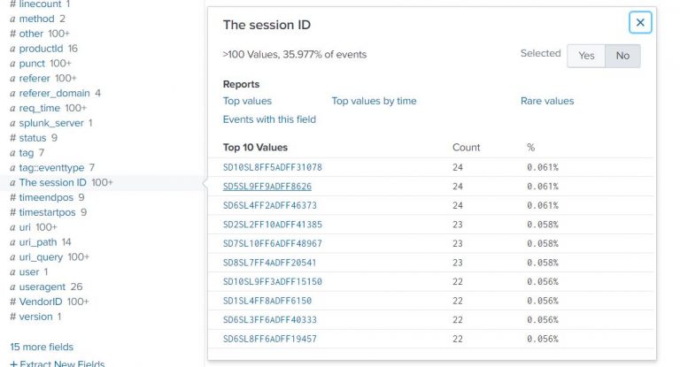
Rename field named JSESSIONID into a human-readable format.
index=test | rename JSESSIONID AS “The session ID” |
Example-2:
Rename the clientip field to “IP Address”.
index=test | rename clientip AS “IP Address” |
Table and fields
The table command is a formatting command and returns a table that is formatted by only the fields that you specify in the arguments. Columns are displayed in the same order that fields are specified. Column headers are the field names. Rows are the field values. Each row represents an event.
The fields command is a filtering command.
The fields command can keep or remove fields from/to the results.
… | fields – A, B – Removes field A and B
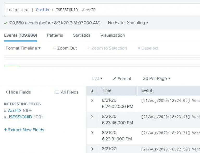
… | fields + A, B – Keeps field A and B and removes all other fields from the results
index=test | fields + JSESSIONID, AcctID |
Sort
The sort command sorts all the results by the specified fields. Results missing a given field are treated as having the smallest or largest possible value of that field if the order is descending or ascending, respectively.
If the first argument to the sort command is a number, then at most that many results are returned in order. If no number is specified, then the default limit of 10000 is used. If the number 0 is specified, then all the results are returned. See the count argument for more information.
By default, the sort command automatically tries to determine what it is sorting. If the field takes on numeric values, the collating sequence is numeric. If the field takes on IP address values, the collating sequence is for IPs. Otherwise, the collating sequence is in lexicographical order.
Some specific examples are:
- Alphabetic strings and punctuation are sorted lexicographically in the UTF-8 encoding order.
- Numeric data is sorted in either ascending or descending order.
- Alphanumeric strings are sorted based on the data type of the first character. If the string starts with a number, then the string is sorted numerically based on that number alone. Otherwise, strings are sorted lexicographically.
- Strings that are a combination of alphanumeric and punctuation characters are sorted the same way as alphanumeric strings.
Example-1:
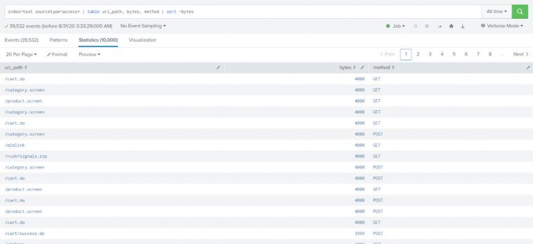
Sort results of web accesses by the request size (descending order).
index=test sourcetype=access* | table uri_path, bytes, method | sort -bytes |
Example-2:
Sort web access data sort in ascending order of HTTP status code.
index=test sourcetype=access* | table uri_path, bytes, method, status | sort status |
Reporting
These commands are used to build transforming searches andreturn statistical data tables that are required for charts and other kinds of data visualizations.
Reporting commands:
- Stats
- Timechart
- Top
Advanced Commands:
- Stats vs eventstats vs streamstats
- Timechart vs chart
Stats
The stats command calculates aggregate statistics such as average, count, and sum, over the results set, similar to SQL aggregation.
If the stats command is used without a BY clause only one row is returned, it is the aggregation over the entire incoming result set. If a BY clause is used, one row is returned for each distinct value specified in the BY clause.
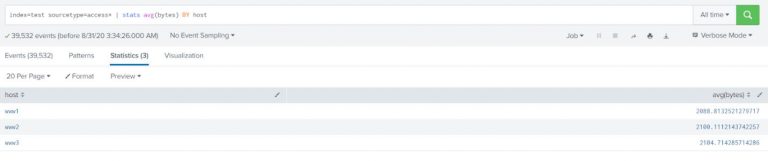
Example-1:
Determine the average request size served in total for each host.
index=test sourcetype=access* | stats avg(bytes) BY host |
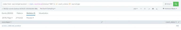
Example-2:
You can also rename the new field to another field name with the stats command.
index=test sourcetype=access* | stats count(eval(status=”404″)) AS count_status BY sourcetype |
Timechart
A timechart is a statistical aggregation applied to a field to produce a chart with time used as the X-axis.
You can specify a split-by field where each distinct value of the split-by field becomes a series in the chart.
The timechart command accepts either the bins OR span argument. If you specify both bins and span, span will be used and the bins argument will be ignored.
If you do not specify either bins or span, the timechart command uses the default bins=100.
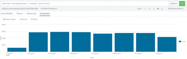
Example-1:
Display column chart over time to show number of requests per day (use web access data, sourcetype=access*).
index=test sourcetype=access* | timechart span=1d count |
See Visualization and select “column chart”
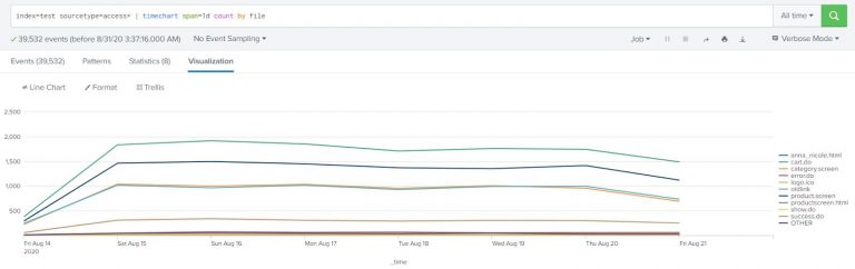
Example-2:
Show the above data with different lines (in a chart) grouped by file. In other words, show the number of requests per file (see field name file) in the same chart.
index=test sourcetype=access* | timechart span=1d count by file |
See visualization and select “line chart”.
Top
Top finds the most common values for the fields in the field list. It calculates a count and a percentage of the frequency the values occur in the events.
If the is included, the results are grouped by the field you specify in the .
- Count – The number of events in your search results that contain the field values that are returned by the top command. See the countfield and showcount arguments.
- Percent – The percentage of events in your search results that contain the field values that are returned by the top command. See the percentfield and showperc arguments.
Example-1:
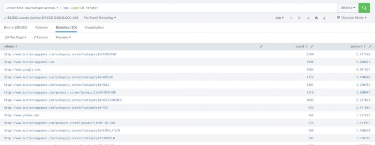
Write a search that returns the 20 most common values of the referer field.
index=test sourcetype=access_* | top limit=20 referer |
The results show the top 20 referer events by count and include the total percentage.
Streamstats
The streamstats command adds cumulative summary statistics to all search results in a streaming manner, calculating statistics for each event at the time the event is seen. For example, you can calculate the running total for a particular field. The total is calculated by using the values in the specified field for every event that has been processed up to the last event.
- Indexing order matters with the output.
- It holds memory of the previous event until it receives a new event.
Example:
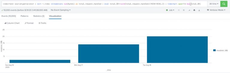
Compute the total request size handled by the server over time (on day 1 the value should be the total of all the requests, on day 2 the size should be the sum of all the requests from both day 1 and day 2).
Use web access data (sourcetype=access*).
index=test sourcetype=access* | sort +_time| streamstats sum(bytes) as total_request_handled | eval total_GB=round(total_request_handled/(1024*1024),2) | timechart span=1d max(total_GB) |
Eventstats
Eventstats generate summary statistics from fields in your events in the same way as the stats command but save the results as a new field instead of displaying them as a table.
- Indexing order does not matter with the output.
- It looks for all the events at a time then computes the result.
Stats vs eventstats
Stats | Eventstats |
Events are transformed into a table of aggregated search results. | Aggregations are placed into a new field that is added to each of the events in your output. |
You can only use the fields in your aggregated results in subsequent commands in the search. | You can use the fields in your events in subsequent commands in your search because the events have not been transformed. |
Example:
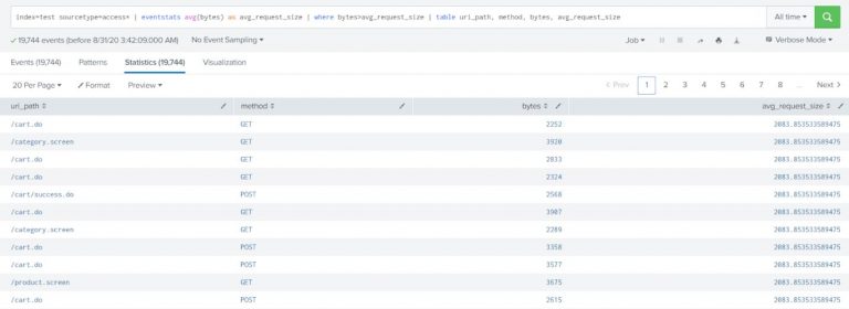
Show all the web access requests which have request size greater than the average size of all the requests.
index=test sourcetype=access* | eventstats avg(bytes) as avg_request_size | where bytes>avg_request_size | table uri_path, method, bytes, avg_request_size |
Correlation commands
These commands are used to build correlation searches. You can combine results from multiple searches and find the correlation between various fields.
Event correlation allows you to find relationships between seemingly unrelated events in data from multiple sources and to help understand which events are most relevant.
Correlation commands:
- Join
- Append
- Appendcol
Advanced Correlation commands:
- Appendpipe
- Map
Join
Use the join command to combine the results of a subsearch with the results of the main search. One or more fields must be in common for each result set.
By default, it performs the inner join. You can override the default value using the type option of the command.
To return matches for one-to-many, many-to-one or many-to-many relationships include the max argument in your join syntax and set the value to 0. By default max=1, which means that the subsearch returns only the first result from the subsearch. Setting the value to a higher number or to 0, which is unlimited, returns multiple results from the subsearch.
Example:
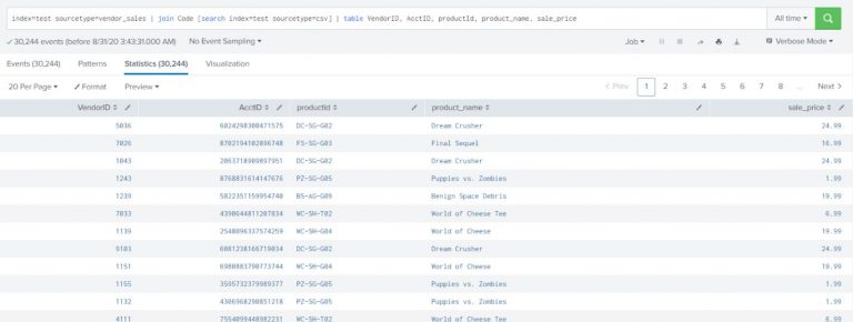
Show vendor information (sourcetype=vendor_sales) with complete product details (details about the product can be found from sourcetype=csv) including product name and price.
index=test sourcetype=vendor_sales | join Code [search index=test sourcetype=csv] | table VendorID, AcctID, productId, product_name, sale_price |
Append
The append command adds the results of a subsearch to the current results. It runs only over historical data and does not produce the correct results if used in a real-time search.
Example-1:
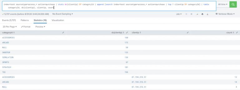
Count the number of different customers who purchased something from the Buttercup Games online store yesterday and display the count for each type of product (accessories, t-shirts, and type of games) they purchased. Also, list the top purchaser for each type of product and how much product that person purchased. Append the top purchaser for each type of product and use the data from the source prices.csv.zip.
index=test sourcetype=access_* action=purchase | stats dc(clientip) BY categoryId | append [search index=test sourcetype=access_* action=purchase | top 1 clientip BY categoryId] | table categoryId, dc(clientip), clientip, count |
Explanation:
In this example, the first searches are for purchase events (action=purchase). These results are piped into the stats command and the dc(), or distinct_count() function is used to count the number of different users who make purchases. The BY clause is used to break up this number based on the different categories of products (category).
This example contains a subsearch as an argument for the append command.
…[search sourcetype=access_* action=purchase | top 1 clientip BY categoryId]
The subsearch is used to search for purchase-related events and counts the top purchaser (based on clientip) for each product category. These results are added to the results of the previous search using the append command.
The table command is used to display only the category of products (categoryId), the distinct count of users who purchased each type of product (dc(clientip)), the actual user who purchased the most of a product type (clientip) and the number of each product that user purchased (count).
Example-2:
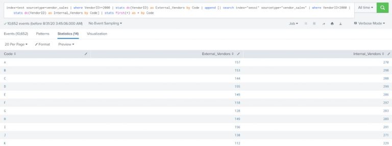
Show the count of distinct internal vendors (VendorID<2000) and count of distinct external vendors (VendorID>=2000) with all the Product Code.
The output should be formatted as listed below:
Code Internal Vendors External Vendors
A 5 4
B 1 3
index=test sourcetype=vendor_sales | where VendorID>=2000 | stats dc(VendorID) as External_Vendors by Code | append [| search index=”sessi” sourcetype=”vendor_sales” | where VendorID<2000 | stats dc(VendorID) as Internal_Vendors by Code] | stats first(*) as * by Code |
Appendpipe
The appendpipe command adds the result of the subpipeline to the search results.
Unlike a subsearch, the subpipeline is not run first – it is run when the search reaches the appendpipe command.
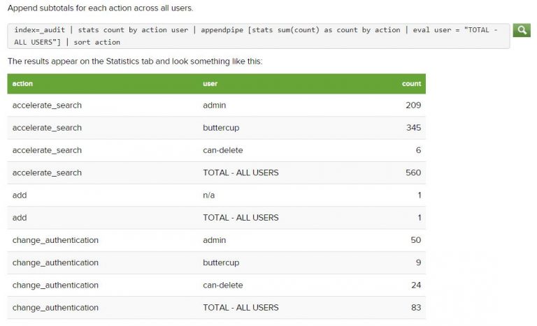
The appendpipe command can be useful because it provides a summary, total, or otherwise descriptive row of the entire dataset when you are constructing a table or chart. This command is also useful when you need the original results for additional calculations.
Example:
Map
The map command is a looping operator that runs a search repeatedly for each input event or result. You can run the map command on a saved search or an ad hoc search but cannot use the map command after an append or appendpipe command in your search pipeline.
Example:
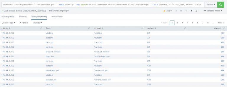
Show the web activity for all IP addresses which have tried accessing the file “passwords.pdf.”
index=test sourcetype=access* file=”passwords.pdf” | dedup clientip | map search=”search index=test sourcetype=access* clientip=$clientip$” | table clientip, file, uri_path, method, status |
Explanation:
The $clientip$ is a token within the search of map command. It will be replaced with the value of clientip field from the result of the first search. So, the search for map command will be executed as many times as the number of results from the first search.
More useful commands
- Predict
- Addinfo (Not explained in the post, Reference)
- Set
- Iplocation
- Geostats
Predict
The predict command forecasts values for one or more sets of time-series data. Additionally, the predict command can fill in missing data in a time-series and can also provide predictions for the next several time steps.
The predict command provides confidence intervals for all its estimates. The command adds a predicted value and an upper and lower 95th percentile range to each event in the time-series.
How the predict command works:
- The predict command models the data by stipulating that there is an unobserved entity that progresses through time in different states.
- To predict a value, the command calculates the best estimate of the state by considering all the data in the past. To compute estimates of the states, the command hypothesizes that the states follow specific linear equations with Gaussian noise components.
- Under this hypothesis, the least-squares estimate of the states is calculated efficiently. This calculation is called the Kalman filter or Kalman-Bucy filter. A confidence interval is obtained for each state estimate. The estimate is not a point estimate but a range of values that contain either the observed or predicted values.
Example:
Predict future access based on the previous access numbers that are stored in Apache web access log files. Count the number of access attempts using a span of one day.
index=test sourcetype=access* | timechart span=1d count(file) as count | predict count |
The results appear on the Statistics tab. Click the Visualization tab. If necessary, change the chart type to a Line Chart.
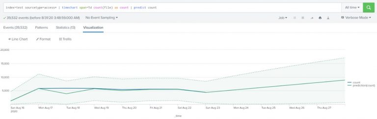
As of machine learning concepts, the more the data the better the prediction. So, if you have data for a longer period of time, then you will have a better prediction.
Set
The set command performs set operations on subsearches.
- Union – Returns a set that combines the results generated by the two subsearches. Provides results that are common to both subsets only once.
- Diff – Returns a set that combines the results generated by the two subsearches and excludes the events common to both. Does not indicate which subsearch the results originated from.
- Intersect – Returns a set that contains results common to both subsearches.
Example:
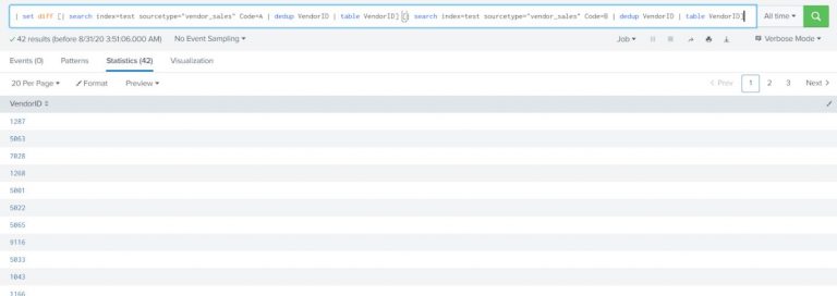
Find all the distinct vendors who purchase item A (Code=A) but not item B.
| set diff [| search index=test sourcetype=”vendor_sales” Code=A | dedup VendorID | table VendorID] [| search index=test sourcetype=”vendor_sales” Code=B | dedup VendorID | table VendorID] |
Iplocation
Iplocation extracts location information from IP addresses by using 3rd-party databases. This command supports IPv4 and IPv6.
The IP address that you specify in the ip-address-fieldname argument is looked up in the database. Fields from that database that contain location information are added to each event. The setting used for the allfields argument determines which fields are added to the events.
Since all the information might not be available for each IP address, an event can have empty field values.
For IP addresses that do not have a location, such as internal addresses, no fields are added.
Example-1:
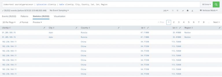
Add location information to web access events. By default, the iplocation command adds the City, Country, lat, lon, and Region fields to the results.
index=test sourcetype=access* | iplocation clientip | table clientip, City, Country, lat, lon, Region |
Example-2:
Search for client errors in web access events, returning only the first 20 results. Add location information and return a table with the IP address, City, and Country for each client error.
index=test sourcetype=access* status>=400 | head 20 | iplocation clientip | table clientip, status, City, Country |
We usually use the iplocation command to get the geolocation and the best way to visualize the geolocation is Map. In that case the geostats command can be used.
Geostats
The fun part is that once you get the geo-location with the iplocation command, you can put the results on a map for a perfect visualization.
The geostats command works in the same fashion as the stats command.
Example:
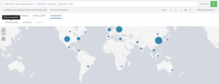
Show the number of requests coming in by different geographical locations on the map (use sourcetype=access*).
index=test sourcetype=access* | iplocation clientip | geostats count |
Choose a Cluster Map for visualization.
Written by Usama Houlila.
Any questions, comments, or feedback are appreciated! Leave a comment or send me an email to uhoulila@cr.jlizardo.com for any questions you might have. Happy Splunking 🙂